Example 1: Time Series Site Response Analysis
This example demonstrates the fundamental concepts of seismic site response analysis using the time series method. We’ll analyze how earthquake ground motion is modified as it propagates through a layered soil profile from bedrock to the surface.
Overview
Time series site response analysis is the most direct approach for studying wave propagation through layered soils. It involves:
Input Motion: Loading a recorded earthquake time series at the bedrock level
Site Model: Defining a layered soil profile with material properties
Wave Propagation: Computing how waves travel upward through the layers
Output Analysis: Examining surface motion and site amplification effects
Key Concepts
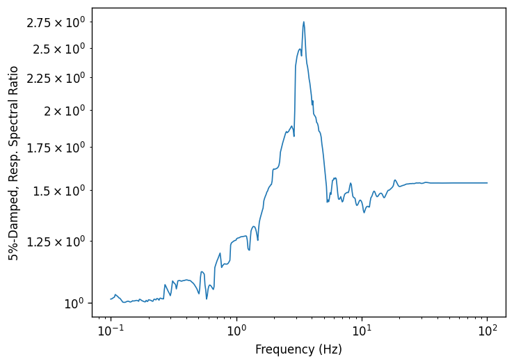
Site Amplification: Soft soils typically amplify seismic waves, especially at frequencies near the site’s natural resonance. This amplification can significantly increase the ground motion intensity compared to bedrock.
Transfer Functions: The relationship between input (bedrock) and output (surface) motion in the frequency domain, showing which frequencies are amplified or attenuated.
Linear vs. Nonlinear: This example uses linear elastic soil behavior, which is appropriate for small to moderate ground motion levels. For strong shaking, nonlinear soil behavior becomes important.
Learning Objectives
After completing this example, you will understand:
How to load earthquake time series data in PyStrata
How to create a simple soil profile
How to run a linear elastic site response analysis
How to interpret response spectra and transfer functions
The physical meaning of site amplification effects
Let’s begin by loading the required packages and data.
[1]:
import matplotlib.pyplot as plt
import numpy as np

import pystrata

%matplotlib inline
[2]:
# Increased figure sizes
plt.rcParams["figure.dpi"] = 120
Load time series data
[3]:
fname = "data/NIS090.AT2"
with open(fname) as fp:
    next(fp)
    description = next(fp).strip()
    next(fp)
    parts = next(fp).split()
    time_step = float(parts[1])

    accels = [float(part) for line in fp for part in line.split()]

    ts = pystrata.motion.TimeSeriesMotion(fname, description, time_step, accels)
[4]:
ts.accels
[4]:
array([2.33833e-07, 2.99033e-07, 5.15835e-07, ..., 4.90601e-05,
       4.94028e-05, 4.96963e-05], shape=(4096,))
There are a few supported file formats. AT2 files can be loaded as follows:
[5]:
ts = pystrata.motion.TimeSeriesMotion.load_at2_file(fname)
ts.accels
[5]:
array([2.33833e-07, 2.99033e-07, 5.15835e-07, ..., 4.90601e-05,
       4.94028e-05, 4.96963e-05], shape=(4096,))
[6]:
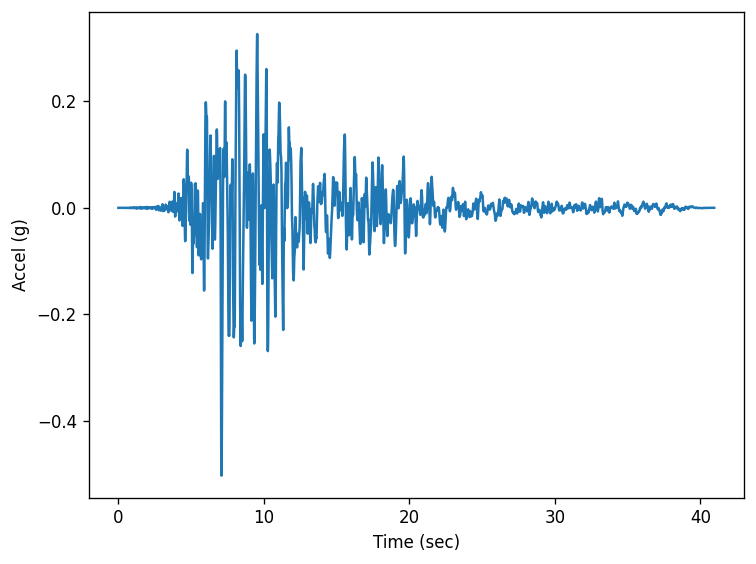
fig, ax = plt.subplots()
ax.plot(ts.times, ts.accels)
ax.set(xlabel="Time (sec)", ylabel="Accel (g)")
fig.tight_layout();
Create site profile
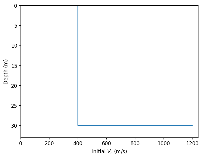
This is about the simplest profile that we can create. Linear-elastic soil and rock.
[7]:
profile = pystrata.site.Profile(
    [
        pystrata.site.Layer(pystrata.site.SoilType("Soil", 18.0, None, 0.05), 30, 400),
        pystrata.site.Layer(pystrata.site.SoilType("Rock", 24.0, None, 0.01), 0, 1200),
    ]
)
[8]:
profile.plot("initial_shear_vel")
[8]:
<Axes: xlabel='Initial $V_s$ (m/s)', ylabel='Depth (m)'>
Create the site response calculator
[9]:
calc = pystrata.propagation.LinearElasticCalculator()
Specify the output
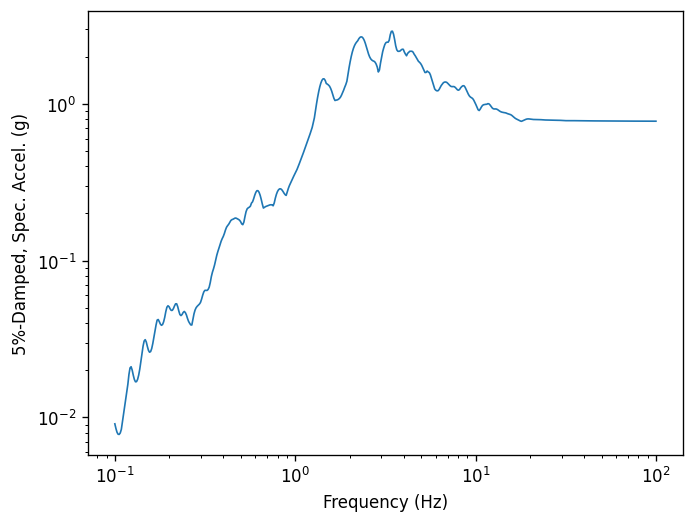
[10]:
freqs = np.logspace(-1, 2, num=500)
outputs = pystrata.output.OutputCollection(
[
pystrata.output.ResponseSpectrumOutput(
# Frequency
freqs,
# Location of the output
pystrata.output.OutputLocation("outcrop", index=0),
# Damping
0.05,
),
pystrata.output.ResponseSpectrumRatioOutput(
# Frequency
freqs,
# Location in (denominator),
pystrata.output.OutputLocation("outcrop", index=-1),
# Location out (numerator)
pystrata.output.OutputLocation("outcrop", index=0),
# Damping
0.05,
),
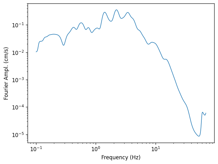
pystrata.output.FourierAmplitudeSpectrumOutput(
# Frequency
freqs,
# Location of the output
pystrata.output.OutputLocation("outcrop", index=0),
# Bandwidth for Konno-Omachi smoothing window
ko_bandwidth=30,
),
]
)
Perform the calculation
Compute the response of the site, and store the state within the calculation object. Nothing is provided.
[11]:
calc(ts, profile, profile.location("outcrop", index=-1))
Calculate all of the outputs from the calculation object.
[12]:
outputs(calc)
Plot the outputs
Create a few plots of the output.
[13]:
for o in outputs:
    o.plot(style="indiv")
[ ]: