Example 6 : TS with Geopsy Profiles

Time series analysis to compute surface response spectrum and site amplification functions using velocity profiles from geopsy.

import re

import matplotlib.pyplot as plt
import numpy as np

import pystrata

%matplotlib inline

# Increased figure sizes
plt.rcParams["figure.dpi"] = 120

Function to parse the geospy files

def iter_geopsy_profiles(fname):
    """Read a Geopsy formatted text file created by gpdcreport."""
    with open(fname) as fp:
        next(fp)
        while True:
            try:
                line = next(fp)
            except StopIteration:
                break

            m = re.search(r"Layered model (\d+): value=([0-9.]+)", line)
            id, score = m.groups()
            count = int(next(fp))
            d = {
                "id": id,
                "score": score,
                "layers": [],
            }
            cols = ["thickness", "vel_comp", "vel_shear", "density"]
            for _ in range(count):
                values = [float(p) for p in next(fp).split()]
                d["layers"].append(dict(zip(cols, values)))

            yield d

Create the input motion

fname = "data/NIS090.AT2"
ts = pystrata.motion.TimeSeriesMotion.load_at2_file(fname)
ts.accels

array([2.33833e-07, 2.99033e-07, 5.15835e-07, ..., 4.90601e-05,
       4.94028e-05, 4.96963e-05], shape=(4096,))

Create the site response calculator

calc = pystrata.propagation.LinearElasticCalculator()

Specify the output

freqs = np.logspace(-1, 2, num=500)

outputs = pystrata.output.OutputCollection(
    [
        pystrata.output.ResponseSpectrumOutput(
            # Frequency
            freqs,
            # Location of the output
            pystrata.output.OutputLocation("outcrop", index=0),
            # Damping
            0.05,
        ),
        pystrata.output.ResponseSpectrumRatioOutput(
            # Frequency
            freqs,
            # Location in (denominator),
            pystrata.output.OutputLocation("outcrop", index=-1),
            # Location out (numerator)
            pystrata.output.OutputLocation("outcrop", index=0),
            # Damping
            0.05,
        ),
    ]
)

Create site profiles

Iterate over the geopsy profiles and create a site profile. For this example, we just use a linear elastic properties.

fname = "data/best100_GM_linux.txt"

for geopsy_profile in iter_geopsy_profiles(fname):
    profile = pystrata.site.Profile(
        [
            pystrata.site.Layer(
                pystrata.site.SoilType(
                    "soil-%d" % i,
                    layer["density"] / pystrata.site.GRAVITY,
                    damping=0.05,
                ),
                layer["thickness"],
                layer["vel_shear"],
            )
            for i, layer in enumerate(geopsy_profile["layers"])
        ]
    )
    # Use 1% damping for the half-space
    profile[-1].soil_type.damping = 0.01
    # Compute the waves from the last layer
    calc(ts, profile, profile.location("outcrop", index=-1))
    # Compute the site amplification
    outputs(calc)

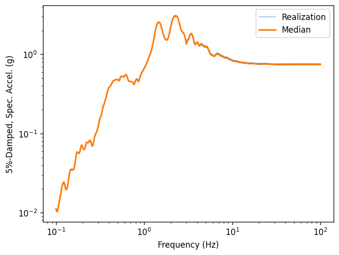
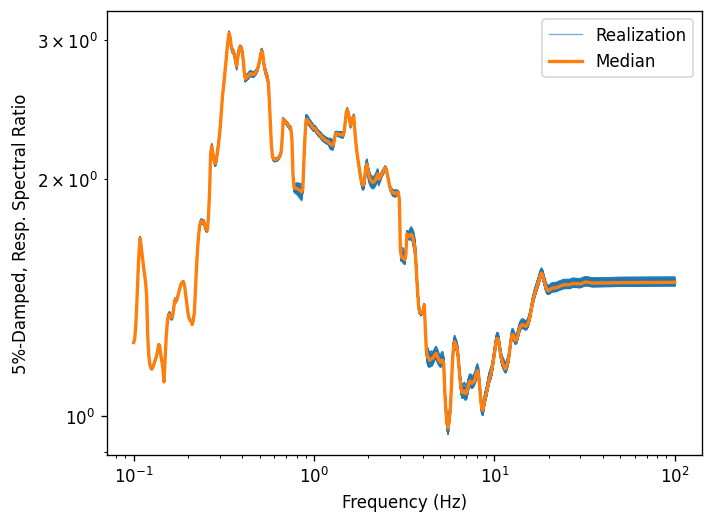
Plot the outputs

Create a few plots of the output.

for o in outputs:
    o.plot(style="stats")