Example 14: RVT SRA with multiple motions and simulated profiles
Example with multiple input motions and simulated soil profiles.
[1]:
import matplotlib.pyplot as plt
import numpy as np
import pandas as pd

import pystrata

%matplotlib inline
[2]:
# Increased figure sizes
plt.rcParams["figure.dpi"] = 120
Create a point source theory RVT motion
[3]:
motions = [
    pystrata.motion.SourceTheoryRvtMotion(5.0, 30, "wna"),
    pystrata.motion.SourceTheoryRvtMotion(6.0, 30, "wna"),
    pystrata.motion.SourceTheoryRvtMotion(7.0, 30, "wna"),
]

for m in motions:
    m.calc_fourier_amps()
Create site profile
This is about the simplest profile that we can create. Linear-elastic soil and rock.
[4]:
profile = pystrata.site.Profile(
    [
        pystrata.site.Layer(
            pystrata.site.DarendeliSoilType(18.0, plas_index=0, ocr=1, stress_mean=100),
            10,
            400,
        ),
        pystrata.site.Layer(
            pystrata.site.DarendeliSoilType(18.0, plas_index=0, ocr=1, stress_mean=200),
            10,
            450,
        ),
        pystrata.site.Layer(
            pystrata.site.DarendeliSoilType(18.0, plas_index=0, ocr=1, stress_mean=400),
            30,
            600,
        ),
        pystrata.site.Layer(pystrata.site.SoilType("Rock", 24.0, None, 0.01), 0, 1200),
    ]
)
Create the site response calculator
[5]:
calc = pystrata.propagation.EquivalentLinearCalculator()
Initialize the variations
[6]:
var_thickness = pystrata.variation.ToroThicknessVariation()
var_velocity = pystrata.variation.DepthDependToroVelVariation.generic_model("USGS C")
var_soiltypes = pystrata.variation.SpidVariation(
    -0.5, std_mod_reduc=0.15, std_damping=0.30
)
Specify the output
[7]:
freqs = np.logspace(-1, 2, num=500)

outputs = pystrata.output.OutputCollection(
    [
        pystrata.output.ResponseSpectrumOutput(
            # Frequency
            freqs,
            # Location of the output
            pystrata.output.OutputLocation("outcrop", index=0),
            # Damping
            0.05,
        ),
        pystrata.output.ResponseSpectrumRatioOutput(
            # Frequency
            freqs,
            # Location in (denominator),
            pystrata.output.OutputLocation("outcrop", index=-1),
            # Location out (numerator)
            pystrata.output.OutputLocation("outcrop", index=0),
            # Damping
            0.05,
        ),
        pystrata.output.InitialVelProfile(),
        pystrata.output.MaxAccelProfile(),
    ]
)
Perform the calculation
[8]:
count = 20
outputs.reset()
for i, p in enumerate(
    pystrata.variation.iter_varied_profiles(
        profile,
        count,
        # var_thickness=var_thickness,
        var_velocity=var_velocity,
        # var_soiltypes=var_soiltypes
    )
):
    # Here we auto-descretize the profile for wave propagation purposes
    p = p.auto_discretize()
    for j, m in enumerate(motions):
        name = (f"p{i}", f"m{j}")
        calc(m, p, p.location("outcrop", index=-1))
        outputs(calc, name=name)
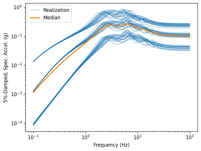
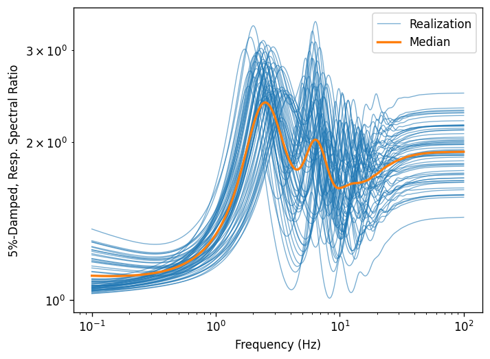
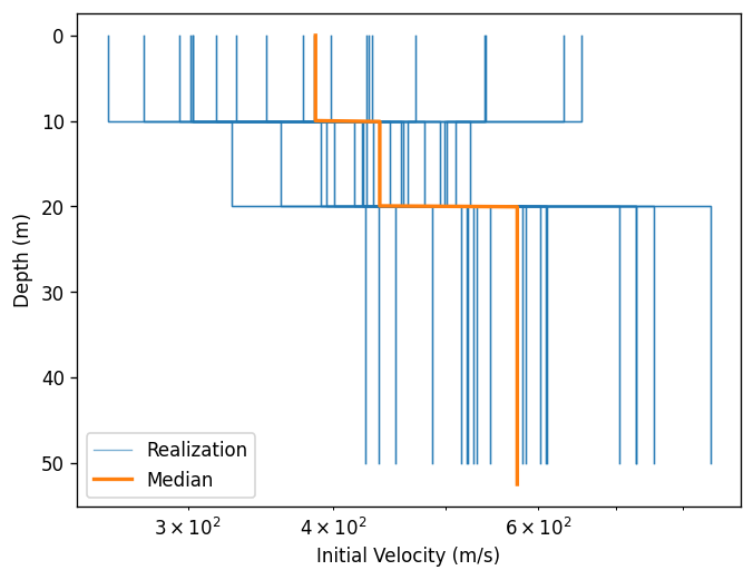
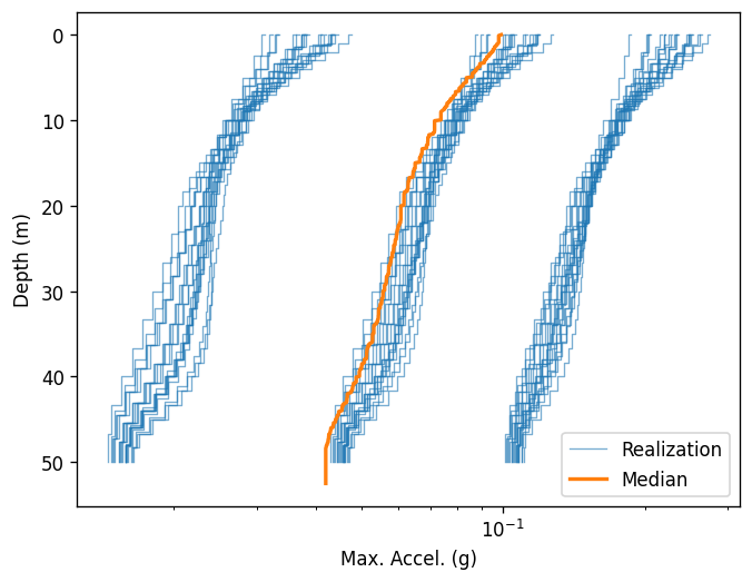
Plot the outputs
Create a few plots of the output.
[9]:
for o in outputs:
    ax = o.plot(style="stats")
Manipulating output as dataframe
If a tuple is passed as the output name, it is used to create a pandas.MultiIndex columns.
[10]:
df = outputs[1].to_dataframe()
df
[10]:
| p0 | p1 | p2 | p3 | ... | p16 | p17 | p18 | p19 | |||||||||||||
|---|---|---|---|---|---|---|---|---|---|---|---|---|---|---|---|---|---|---|---|---|---|
| m0 | m1 | m2 | m0 | m1 | m2 | m0 | m1 | m2 | m0 | ... | m2 | m0 | m1 | m2 | m0 | m1 | m2 | m0 | m1 | m2 | |
| 0.100000 | 1.199169 | 1.067144 | 1.041937 | 1.365337 | 1.114246 | 1.070332 | 1.150166 | 1.052062 | 1.032794 | 1.160323 | ... | 1.051661 | 1.218265 | 1.074727 | 1.047878 | 1.247118 | 1.081724 | 1.051042 | 1.237391 | 1.080083 | 1.050872 |
| 0.101394 | 1.198486 | 1.067095 | 1.042262 | 1.363797 | 1.114110 | 1.070849 | 1.149752 | 1.052039 | 1.033056 | 1.159850 | ... | 1.052056 | 1.217541 | 1.074669 | 1.048245 | 1.246198 | 1.081650 | 1.051430 | 1.236558 | 1.080015 | 1.051258 |
| 0.102807 | 1.197805 | 1.067050 | 1.042591 | 1.362262 | 1.113982 | 1.071373 | 1.149340 | 1.052019 | 1.033320 | 1.159379 | ... | 1.052455 | 1.216819 | 1.074617 | 1.048616 | 1.245280 | 1.081581 | 1.051823 | 1.235727 | 1.079952 | 1.051649 |
| 0.104240 | 1.197127 | 1.067011 | 1.042924 | 1.360731 | 1.113860 | 1.071902 | 1.148929 | 1.052004 | 1.033587 | 1.158909 | ... | 1.052859 | 1.216099 | 1.074569 | 1.048990 | 1.244366 | 1.081519 | 1.052219 | 1.234899 | 1.079894 | 1.052044 |
| 0.105693 | 1.196451 | 1.066976 | 1.043259 | 1.359205 | 1.113746 | 1.072437 | 1.148519 | 1.051993 | 1.033856 | 1.158442 | ... | 1.053267 | 1.215383 | 1.074528 | 1.049368 | 1.243456 | 1.081462 | 1.052620 | 1.234075 | 1.079843 | 1.052442 |
| ... | ... | ... | ... | ... | ... | ... | ... | ... | ... | ... | ... | ... | ... | ... | ... | ... | ... | ... | ... | ... | ... |
| 94.613238 | 1.890833 | 1.816821 | 1.708854 | 2.159850 | 2.004552 | 1.740940 | 2.149550 | 2.031974 | 1.954668 | 1.983983 | ... | 1.437305 | 2.294969 | 2.155980 | 2.013320 | 2.019502 | 1.920447 | 1.765683 | 2.199050 | 2.077446 | 1.926454 |
| 95.932095 | 1.890908 | 1.816891 | 1.708942 | 2.159961 | 2.004677 | 1.741084 | 2.149588 | 2.032002 | 1.954720 | 1.984042 | ... | 1.437417 | 2.295040 | 2.156050 | 2.013423 | 2.019583 | 1.920530 | 1.765787 | 2.199132 | 2.077527 | 1.926563 |
| 97.269336 | 1.890981 | 1.816958 | 1.709027 | 2.160067 | 2.004799 | 1.741225 | 2.149624 | 2.032029 | 1.954771 | 1.984099 | ... | 1.437526 | 2.295109 | 2.156117 | 2.013522 | 2.019662 | 1.920611 | 1.765888 | 2.199212 | 2.077605 | 1.926668 |
| 98.625218 | 1.891051 | 1.817024 | 1.709109 | 2.160171 | 2.004917 | 1.741361 | 2.149659 | 2.032055 | 1.954820 | 1.984154 | ... | 1.437632 | 2.295175 | 2.156182 | 2.013618 | 2.019738 | 1.920688 | 1.765985 | 2.199289 | 2.077681 | 1.926770 |
| 100.000000 | 1.891119 | 1.817087 | 1.709189 | 2.160271 | 2.005032 | 1.741492 | 2.149694 | 2.032080 | 1.954867 | 1.984207 | ... | 1.437735 | 2.295240 | 2.156245 | 2.013712 | 2.019812 | 1.920764 | 1.766080 | 2.199363 | 2.077755 | 1.926869 |
500 rows × 60 columns
Lets names to the dataframe and transform into a long format. Pandas works better on long formatted tables.
[11]:
# Add names for clarity
df.columns.names = ("profile", "motion")
df.index.name = "freq"
# Transform into a long format
df = df.melt(ignore_index=False).reset_index().set_index(["freq", "profile", "motion"])
df
[11]:
| value | |||
|---|---|---|---|
| freq | profile | motion | |
| 0.100000 | p0 | m0 | 1.199169 |
| 0.101394 | p0 | m0 | 1.198486 |
| 0.102807 | p0 | m0 | 1.197805 |
| 0.104240 | p0 | m0 | 1.197127 |
| 0.105693 | p0 | m0 | 1.196451 |
| ... | ... | ... | ... |
| 94.613238 | p19 | m2 | 1.926454 |
| 95.932095 | p19 | m2 | 1.926563 |
| 97.269336 | p19 | m2 | 1.926668 |
| 98.625218 | p19 | m2 | 1.926770 |
| 100.000000 | p19 | m2 | 1.926869 |
30000 rows × 1 columns
[12]:
def calc_stats(group):
    ln_value = np.log(group["value"])

    median = np.exp(np.mean(ln_value))
    ln_std = np.std(ln_value)

    return pd.Series({"median": median, "ln_std": ln_std})


stats = df.groupby(level=["freq", "motion"]).apply(calc_stats)
stats
[12]:
| median | ln_std | ||
|---|---|---|---|
| freq | motion | ||
| 0.100000 | m0 | 1.221754 | 0.048237 |
| m1 | 1.074200 | 0.016712 | |
| m2 | 1.046574 | 0.010814 | |
| 0.101394 | m0 | 1.220970 | 0.048028 |
| m1 | 1.074139 | 0.016685 | |
| ... | ... | ... | ... |
| 98.625218 | m1 | 1.932465 | 0.101221 |
| m2 | 1.793673 | 0.098151 | |
| 100.000000 | m0 | 2.036655 | 0.115260 |
| m1 | 1.932532 | 0.101219 | |
| m2 | 1.793761 | 0.098149 |
1500 rows × 2 columns
[13]:
stats = (
    stats.reset_index("motion")
    .pivot(columns="motion")
    .swaplevel(0, 1, axis=1)
    .sort_index(axis=1)
)
stats
[13]:
| motion | m0 | m1 | m2 | |||
|---|---|---|---|---|---|---|
| ln_std | median | ln_std | median | ln_std | median | |
| freq | ||||||
| 0.100000 | 0.048237 | 1.221754 | 0.016712 | 1.074200 | 0.010814 | 1.046574 |
| 0.101394 | 0.048028 | 1.220970 | 0.016685 | 1.074139 | 0.010885 | 1.046931 |
| 0.102807 | 0.047820 | 1.220189 | 0.016659 | 1.074082 | 0.010957 | 1.047290 |
| 0.104240 | 0.047611 | 1.219411 | 0.016633 | 1.074031 | 0.011029 | 1.047654 |
| 0.105693 | 0.047404 | 1.218636 | 0.016608 | 1.073986 | 0.011102 | 1.048022 |
| ... | ... | ... | ... | ... | ... | ... |
| 94.613238 | 0.115272 | 2.036368 | 0.101226 | 1.932250 | 0.098159 | 1.793393 |
| 95.932095 | 0.115269 | 2.036443 | 0.101224 | 1.932324 | 0.098156 | 1.793490 |
| 97.269336 | 0.115266 | 2.036516 | 0.101223 | 1.932396 | 0.098154 | 1.793583 |
| 98.625218 | 0.115263 | 2.036586 | 0.101221 | 1.932465 | 0.098151 | 1.793673 |
| 100.000000 | 0.115260 | 2.036655 | 0.101219 | 1.932532 | 0.098149 | 1.793761 |
500 rows × 6 columns
Access the properties of each motion like:
[14]:
stats["m0"]
[14]:
| ln_std | median | |
|---|---|---|
| freq | ||
| 0.100000 | 0.048237 | 1.221754 |
| 0.101394 | 0.048028 | 1.220970 |
| 0.102807 | 0.047820 | 1.220189 |
| 0.104240 | 0.047611 | 1.219411 |
| 0.105693 | 0.047404 | 1.218636 |
| ... | ... | ... |
| 94.613238 | 0.115272 | 2.036368 |
| 95.932095 | 0.115269 | 2.036443 |
| 97.269336 | 0.115266 | 2.036516 |
| 98.625218 | 0.115263 | 2.036586 |
| 100.000000 | 0.115260 | 2.036655 |
500 rows × 2 columns
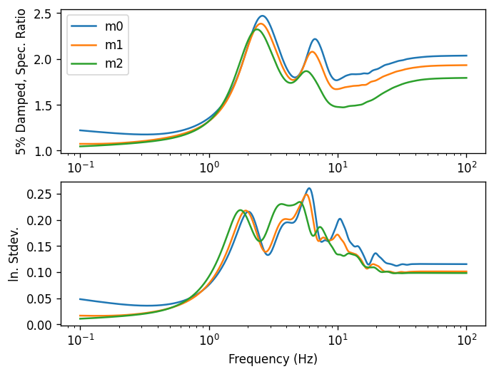
[15]:
fig, axes = plt.subplots(nrows=2, subplot_kw={"xscale": "log"})

for name, g in stats.T.groupby(level=0):
    for ax, key in zip(axes, ["median", "ln_std"]):
        ax.plot(g.columns, g.loc[name, key], label=name)


axes[0].set(ylabel="5% Damped, Spec. Ratio")
axes[0].legend()

axes[1].set(ylabel="ln. Stdev.", xlabel="Frequency (Hz)")

fig;