Example 2: Random vibration theory SRA

Random vibration theory analysis to compute surface response spectrum and site amplification functions.

import matplotlib.pyplot as plt
import numpy as np

import pystrata

%matplotlib inline

# Increased figure sizes
plt.rcParams["figure.dpi"] = 120

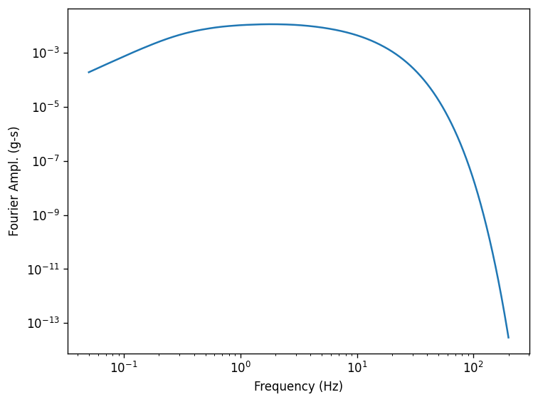
Create a point source theory RVT motion

m = pystrata.motion.SourceTheoryRvtMotion(6.0, 30, "wna")
m.calc_fourier_amps()

fig, ax = plt.subplots()
ax.plot(m.freqs, m.fourier_amps)
ax.set(
    xlabel="Frequency (Hz)", xscale="log", ylabel="Fourier Ampl. (g-s)", yscale="log"
)
fig.tight_layout();

Create site profile

This is about the simplest profile that we can create. Linear-elastic soil and rock.

profile = pystrata.site.Profile(
    [
        pystrata.site.Layer(pystrata.site.SoilType("Soil", 18.0, None, 0.05), 30, 400),
        pystrata.site.Layer(pystrata.site.SoilType("Rock", 24.0, None, 0.01), 0, 1200),
    ]
)

Create the site response calculator

calc = pystrata.propagation.LinearElasticCalculator()

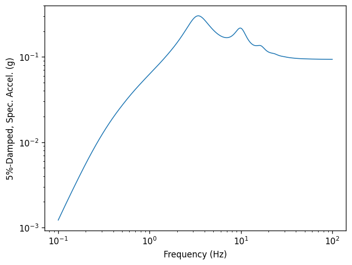
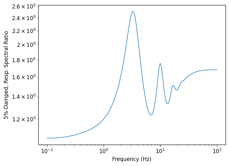
Specify the output

freqs = np.logspace(-1, 2, num=500)

outputs = pystrata.output.OutputCollection(
    [
        pystrata.output.ResponseSpectrumOutput(
            # Frequency
            freqs,
            # Location of the output
            pystrata.output.OutputLocation("outcrop", index=0),
            # Damping
            0.05,
        ),
        pystrata.output.ResponseSpectrumRatioOutput(
            # Frequency
            freqs,
            # Location in (denominator),
            pystrata.output.OutputLocation("outcrop", index=-1),
            # Location out (numerator)
            pystrata.output.OutputLocation("outcrop", index=0),
            # Damping
            0.05,
        ),
    ]
)

Perform the calculation

Compute the response of the site, and store the state within the calculation object. Nothing is provided.

calc(m, profile, profile.location("outcrop", index=-1))

Calculate all of the outputs from the calculation object.

outputs(calc)

Plot the outputs

Create a few plots of the output.

for o in outputs:
    o.plot(style="indiv")