Example 4: Simulated site profile

Generate simulated shear-wave velocity profiles.

import matplotlib.pyplot as plt

import pystrata

%matplotlib inline

# Increased figure sizes
plt.rcParams["figure.dpi"] = 120

Create a simple site profile

profile = pystrata.site.Profile(
    [
        pystrata.site.Layer(
            pystrata.site.SoilType("Soil-1", 18.0, None, 0.05), 30, 400
        ),
        pystrata.site.Layer(
            pystrata.site.SoilType("Soil-2", 19.0, None, 0.05), 20, 600
        ),
        pystrata.site.Layer(pystrata.site.SoilType("Rock", 24.0, None, 0.01), 0, 1200),
    ]
)

Initialize the variations.

toro_thickness = pystrata.variation.ToroThicknessVariation()
toro_velocity = pystrata.variation.ToroVelocityVariation.generic_model("USGS B")

Create the varied thickness and velocity.

%pdb

Automatic pdb calling has been turned ON

count = 10
# Create realizations of the profile with varied thickness
varied_thick = [toro_thickness(profile) for _ in range(count)]

# For eaach realization of varied thickness, vary the shear-wave velocity
varied_vel = [toro_velocity(rt) for rt in varied_thick]

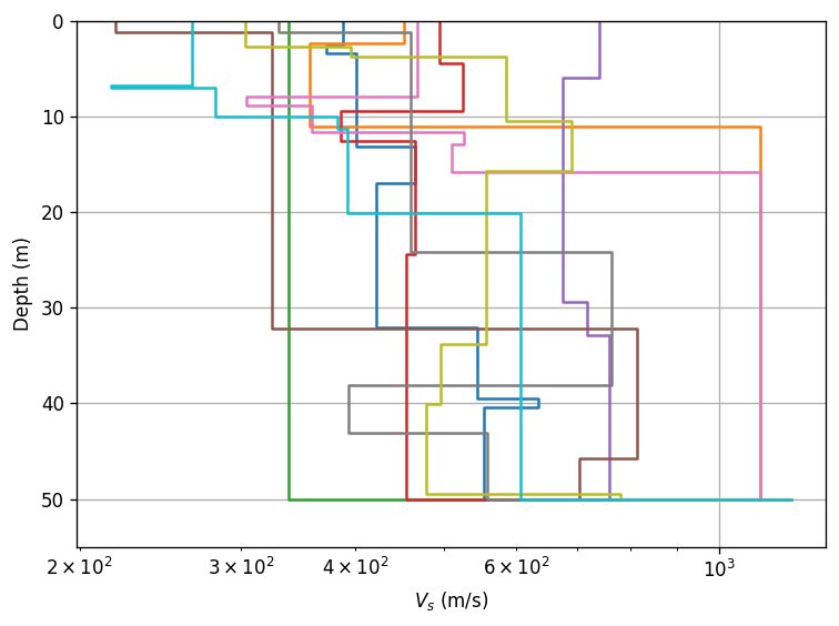
Create a plot of the varied velocity models.

fig, ax = plt.subplots()

for profile in varied_vel:
    ax.plot(
        [layer.initial_shear_vel for layer in profile],
        [layer.depth for layer in profile],
        drawstyle="steps-pre",
    )

ax.set(xlabel="$V_s$ (m/s)", xscale="log", ylabel="Depth (m)", ylim=(55, 0))

ax.grid()
fig.tight_layout();

Example of varying bedrock depth

Setup

# Import to specify distribution of bedrock depth
from scipy.stats import uniform

# Parameters for distribution of bedrock depth
depth_bedrock = 50
depth_bedrock_min = 40
depth_bedrock_max = 65
uniform_dist_loc = depth_bedrock_min
uniform_dist_scale = depth_bedrock_max - depth_bedrock_min
uniform_dist = uniform(loc=uniform_dist_loc, scale=uniform_dist_scale)

# Parameters for distribution of velocities
PARAMS = {
    "USGS B": {  # To be consistent with example above
        "ln_std": 0.27,
        "rho_0": 0.97,
        "delta": 3.8,
        "rho_200": 1.00,
        "h_0": 0.0,
        "b": 0.293,
    }
}

Initialize instances of classes for randomizing profiles

var_bedrock = pystrata.variation.HalfSpaceDepthVariation(dist=uniform_dist)

var_thickness = pystrata.variation.ToroThicknessVariation()

var_velocity = pystrata.variation.ToroVelocityVariation(
    ln_std=PARAMS["USGS B"]["ln_std"],
    rho_0=PARAMS["USGS B"]["rho_0"],
    delta=PARAMS["USGS B"]["delta"],
    rho_200=PARAMS["USGS B"]["rho_200"],
    h_0=PARAMS["USGS B"]["h_0"],
    b=PARAMS["USGS B"]["b"],
    vary_bedrock=True,  # Enable variation of bedrock depth
)

Randomize soil profiles

num_sim = 3

# Create realizations of the profile with varied bedrock depths
varied_depths = [var_bedrock(profile) for _ in range(num_sim)]

# For each realization of varied depth, vary the thicknesses
varied_thicknesses = [var_thickness(rd) for rd in varied_depths]

# For each realization of varied thicknesses, vary the velocities
varied_velocities = [var_velocity(rt) for rt in varied_thicknesses]

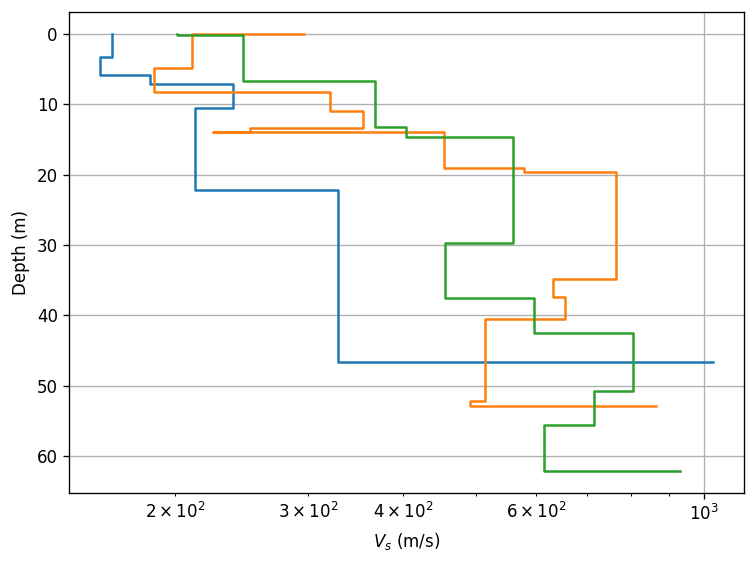
Plot randomized profiles

fig, ax = plt.subplots()

for profile in varied_velocities:
    ax.plot(
        [layer.initial_shear_vel for layer in profile],
        [layer.depth for layer in profile],
        drawstyle="steps-pre",
    )

ax.invert_yaxis()
ax.set(xlabel="$V_s$ (m/s)", xscale="log", ylabel="Depth (m)")

ax.grid()
fig.tight_layout();