Example 11 : Time series SRA using FDM

Time series analysis to acceleration transfer functions and spectral ratios.

import matplotlib.pyplot as plt
import numpy as np

import pystrata

%matplotlib inline

# Increased figure sizes
plt.rcParams["figure.dpi"] = 120

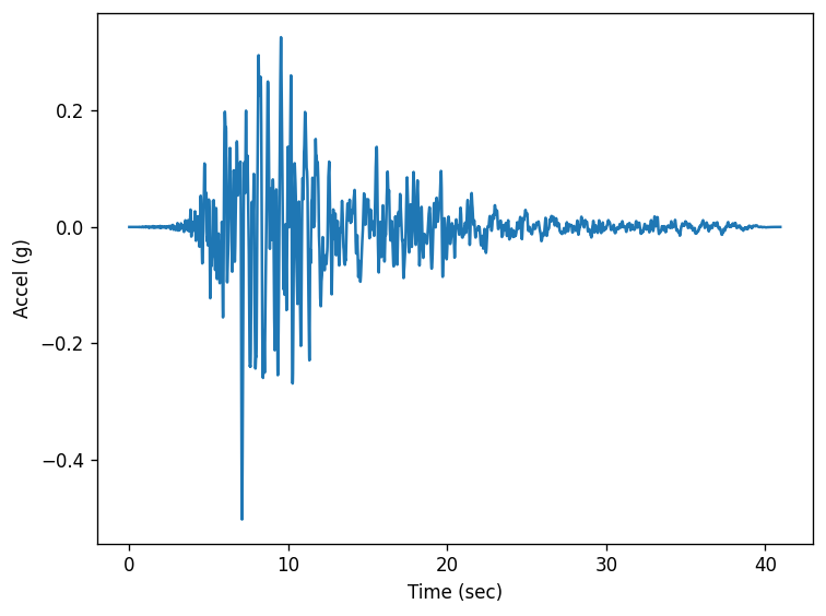
Load time series data

fname = "data/NIS090.AT2"
with open(fname) as fp:
    next(fp)
    description = next(fp).strip()
    next(fp)
    parts = next(fp).split()
    time_step = float(parts[1])

    accels = [float(part) for line in fp for part in line.split()]

    ts = pystrata.motion.TimeSeriesMotion(fname, description, time_step, accels)

ts.accels

array([2.33833e-07, 2.99033e-07, 5.15835e-07, ..., 4.90601e-05,
       4.94028e-05, 4.96963e-05], shape=(4096,))

There are a few supported file formats. AT2 files can be loaded as follows:

ts = pystrata.motion.TimeSeriesMotion.load_at2_file(fname)
ts.accels

array([2.33833e-07, 2.99033e-07, 5.15835e-07, ..., 4.90601e-05,
       4.94028e-05, 4.96963e-05], shape=(4096,))

fig, ax = plt.subplots()
ax.plot(ts.times, ts.accels)
ax.set(xlabel="Time (sec)", ylabel="Accel (g)")
fig.tight_layout();

Create site profile

This is about the simplest profile that we can create. Linear-elastic soil and rock.

profile = pystrata.site.Profile(
    [
        pystrata.site.Layer(
            pystrata.site.DarendeliSoilType(18.0, plas_index=0, ocr=1, stress_mean=200),
            30,
            400,
        ),
        pystrata.site.Layer(pystrata.site.SoilType("Rock", 24.0, None, 0.01), 0, 1200),
    ]
)

Create the site response calculator

calcs = [
    ("EQL", pystrata.propagation.EquivalentLinearCalculator()),
    (
        "FDM (KA)",
        pystrata.propagation.FrequencyDependentEqlCalculator(
            strain_ratio=0.65, method="ka02"
        ),
    ),
    (
        "FDM (ZR)",
        pystrata.propagation.FrequencyDependentEqlCalculator(method="zr15"),
    ),
    (
        "FDM (KO 0.3)",
        pystrata.propagation.FrequencyDependentEqlCalculator(method="ko:20"),
    ),
]

Specify the output

freqs = np.logspace(-1, np.log10(50.0), num=500)

outputs = pystrata.output.OutputCollection(
    [
        pystrata.output.ResponseSpectrumOutput(
            # Frequency
            freqs,
            # Location of the output
            pystrata.output.OutputLocation("outcrop", index=0),
            # Damping
            0.05,
        ),
        pystrata.output.ResponseSpectrumRatioOutput(
            # Frequency
            freqs,
            # Location in (denominator),
            pystrata.output.OutputLocation("outcrop", index=-1),
            # Location out (numerator)
            pystrata.output.OutputLocation("outcrop", index=0),
            # Damping
            0.05,
        ),
        pystrata.output.AccelTransferFunctionOutput(
            # Frequency
            freqs,
            # Location in (denominator),
            pystrata.output.OutputLocation("outcrop", index=-1),
            # Location out (numerator)
            pystrata.output.OutputLocation("outcrop", index=0),
        ),
        pystrata.output.AccelTransferFunctionOutput(
            # Frequency
            freqs,
            # Location in (denominator),
            pystrata.output.OutputLocation("outcrop", index=-1),
            # Location out (numerator)
            pystrata.output.OutputLocation("outcrop", index=0),
            ko_bandwidth=30,
        ),
    ]
)

Perform the calculation

Compute the response of the site, and store the state within the calculation object, which is then used along with the output collection to compute the desired outputs. Also, extract the computed properties for comparison.

properties = {}
for name, calc in calcs:
    calc(ts, profile, profile.location("outcrop", index=-1))
    outputs(calc, name)

    properties[name] = {
        key: getattr(profile[0], key) for key in ["shear_mod_reduc", "damping"]
    }

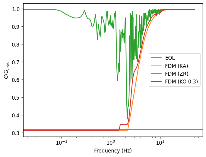
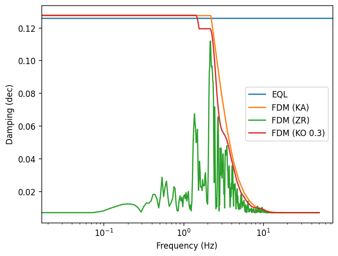
Plot the final properties

for key in properties["EQL"].keys():
    fig, ax = plt.subplots()

    for i, (k, p) in enumerate(properties.items()):
        if k == "EQL":
            ax.axhline(p[key], label=k, color=f"C{i}")
        else:
            ax.plot(ts.freqs, p[key], label=k, color=f"C{i}")

    ax.set(
        ylabel={"damping": "Damping (dec)", "shear_mod_reduc": r"$G/G_{max}$"}[key],
        xlabel="Frequency (Hz)",
        xscale="log",
    )
    ax.legend()

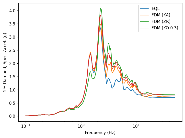
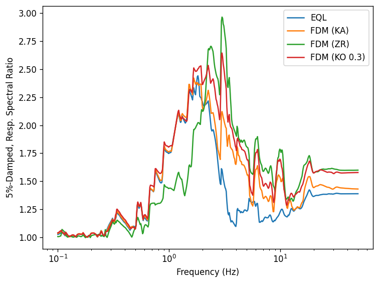
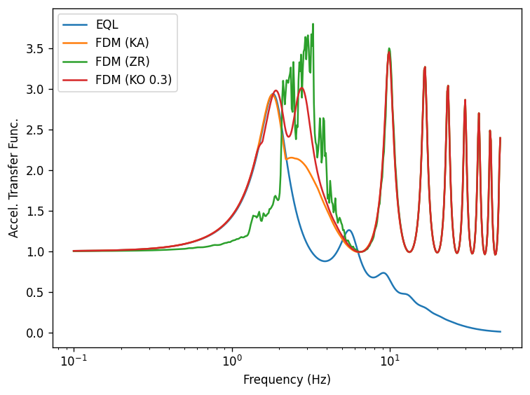
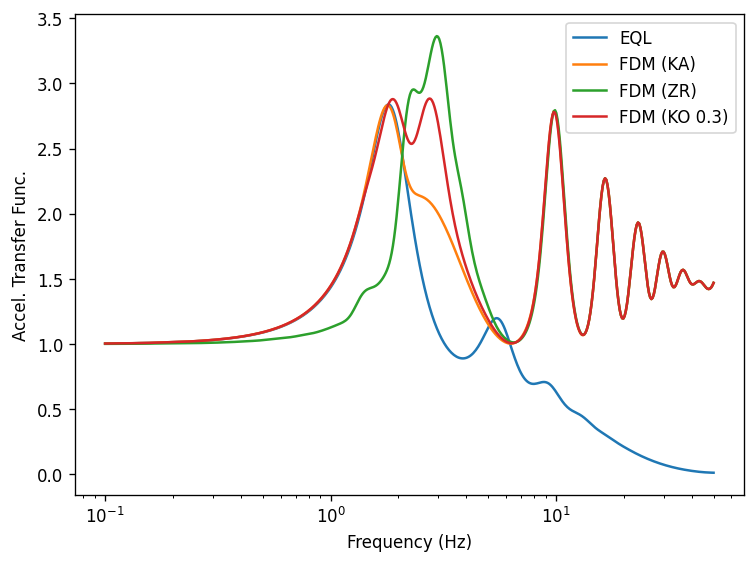
Plot the outputs

Create a few plots of the output.

for output in outputs:
    fig, ax = plt.subplots()
    for name, refs, values in output.iter_results():
        ax.plot(refs, values, label=name)

    ax.set(xlabel=output.xlabel, xscale="log", ylabel=output.ylabel)
    ax.legend()
    fig.tight_layout()