Example 9: Quarter wavelength site amplification

Example of quarter-wavelength site amplification and fitting a profile to a target crustal amplification.

import json

import matplotlib.pyplot as plt
import numpy as np

import pystrata

%matplotlib inline

# Increased figure sizes
plt.rcParams["figure.dpi"] = 120

Load the WNA profile from Campbell (2003).

with open("../tests/data/qwl_tests.json") as fp:
    data = json.load(fp)[1]

thickness = np.diff(data["site"]["depth"])

profile = pystrata.site.Profile()
for i, (thick, vel_shear, density) in enumerate(
    zip(thickness, data["site"]["velocity"], data["site"]["density"])
):
    profile.append(
        pystrata.site.Layer(
            pystrata.site.SoilType(f"{i}", density * pystrata.motion.GRAVITY),
            thick * 1000,
            vel_shear * 1000,
        )
    )

profile.update_layers(0)

Create simple point source motion

motion = pystrata.motion.SourceTheoryRvtMotion(
    magnitude=6.5, distance=20, region="cena"
)
motion.calc_fourier_amps(data["freqs"])

calc = pystrata.propagation.QuarterWaveLenCalculator(site_atten=0.04)
input_loc = profile.location("outcrop", index=-1)

calc(motion, profile, input_loc)

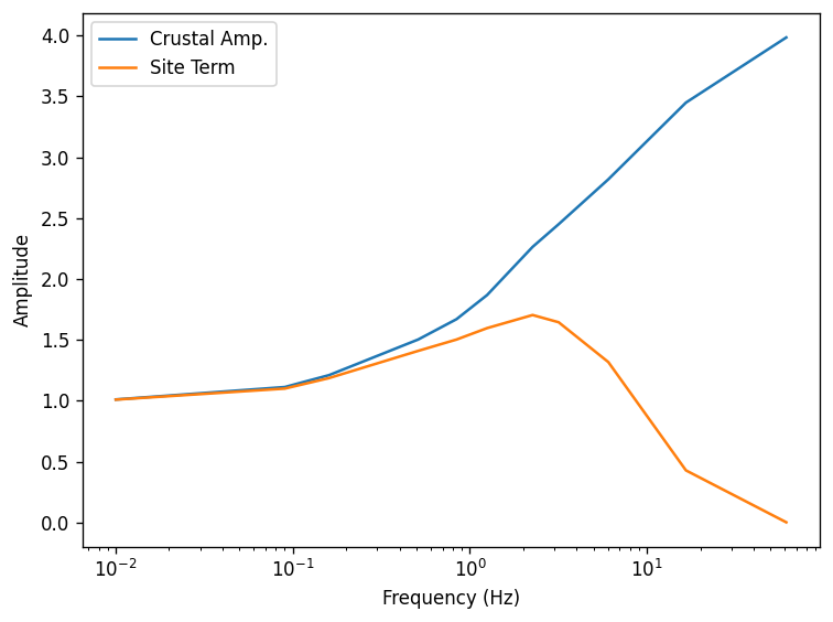
fig, ax = plt.subplots()
ax.plot(motion.freqs, calc.crustal_amp, label="Crustal Amp.")
ax.plot(motion.freqs, calc.site_term, label="Site Term")
ax.set(
    xlabel="Frequency (Hz)",
    xscale="log",
    ylabel="Amplitude",
    yscale="linear",
)
ax.legend()
fig.tight_layout();

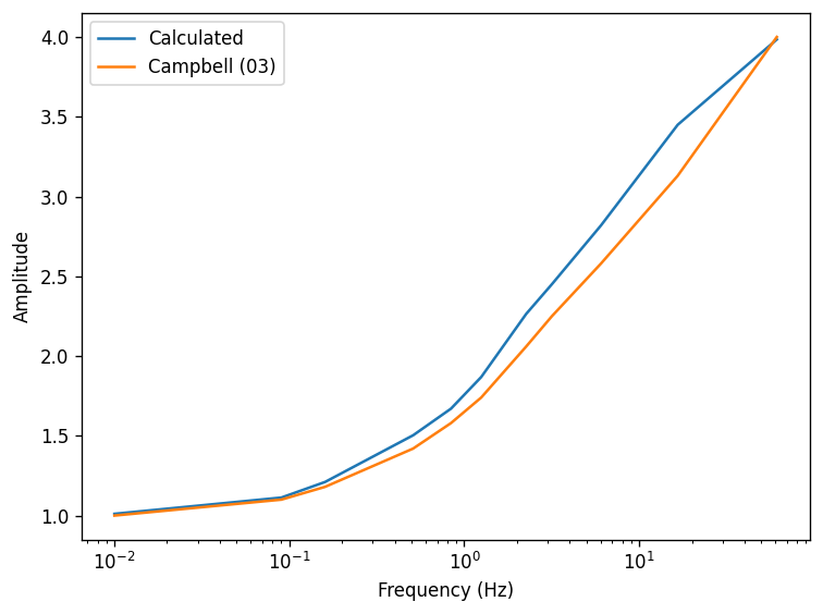
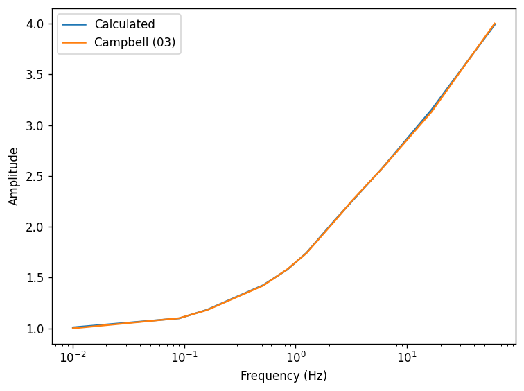
The quarter-wavelength calculation is tested against the WNA and CENA crustal amplification models provided by Campbell (2003). The test of the CENA model passes, but the WNA model fails. Below is a comparison of the two crustal amplifications.

fig, ax = plt.subplots()
ax.plot(motion.freqs, calc.crustal_amp, label="Calculated")
ax.plot(data["freqs"], data["crustal_amp"], label="Campbell (03)")
ax.set(
    xlabel="Frequency (Hz)",
    xscale="log",
    ylabel="Amplitude",
    yscale="linear",
)
ax.legend()
fig.tight_layout();

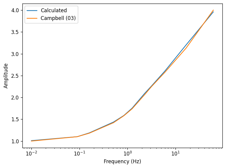
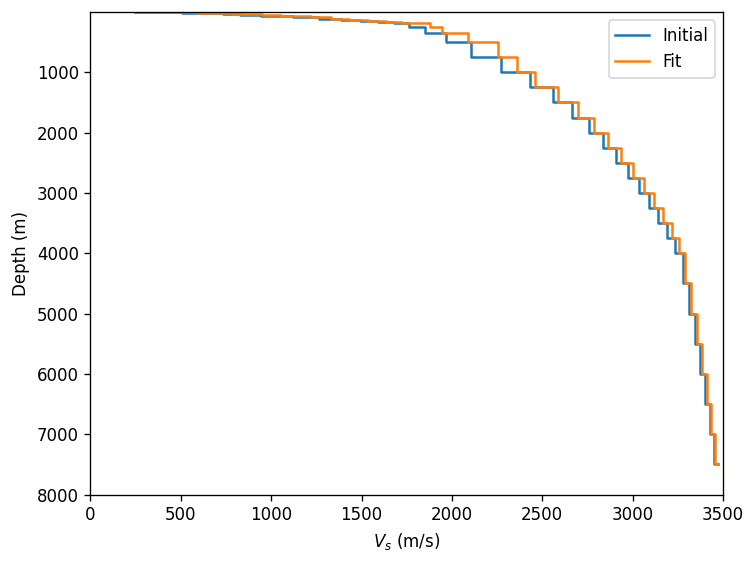
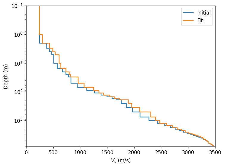
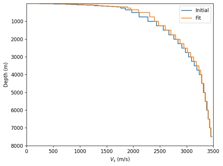
Adjust the profile to match the target crustal amplification – no consideration of the site attenuation paramater although this can also be done. First, the adjustment is only performed on the velocity. Second set of plots adjusts velocity and thickness.

for adjust_thickness in [False, True]:
    calc.fit(
        target_type="crustal_amp",
        target=data["crustal_amp"],
        adjust_thickness=adjust_thickness,
    )

    fig, ax = plt.subplots()
    ax.plot(motion.freqs, calc.crustal_amp, label="Calculated")
    ax.plot(data["freqs"], data["crustal_amp"], label="Campbell (03)")
    ax.set(
        xlabel="Frequency (Hz)",
        xscale="log",
        ylabel="Amplitude",
        yscale="linear",
    )
    ax.legend()
    fig.tight_layout()

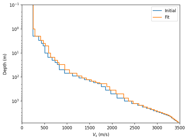
    for yscale in ["log", "linear"]:
        fig, ax = plt.subplots()

        ax.plot(
            profile.initial_shear_vel,
            profile.depth,
            label="Initial",
            drawstyle="steps-pre",
        )
        ax.plot(
            calc.profile.initial_shear_vel,
            calc.profile.depth,
            label="Fit",
            drawstyle="steps-pre",
        )

        ax.legend()
        ax.set(
            xlabel="$V_s$ (m/s)",
            xlim=(0, 3500),
            ylabel="Depth (m)",
            ylim=(8000, 0.1),
            yscale=yscale,
        )
        fig.tight_layout()